Conditional Formatting.
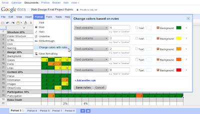
Take advantage of a lesser known Google Docs Spreadsheet function – “Change colors with rules…” to view data “horizontally” and “vertically.” For this particular rubric, I highlighted the students’ scores and set the numbers 0, 1, 2, 3, and 4 to Red, Orange, Light Orange, Yellow, and Green respectively. See below.
Sample
View a sample conditionally formatted rubric.
The Result?
At just a quick “horizontal” glance, it is easy to see among the field of green (which means 4 or full credit) that students struggled with the design requirement more than any other. Reteaching should focus in this area.
A quick “vertical” glance reveals a lot of red and orange for student 15. Additional support, and possible intervention, should be provided to this student.
Give this a try, and comment below to let me know how this worked for you.